In this tutorial we will learn some basic image manipulation operations using the OpenCV library.
The images used are available as educational resources on the page: http://www.imageprocessingplace.com/DIP-3E/dip3e_book_images_downloads.htm
Libraries and packages
import cv2

import matplotlib.pyplot as plt

import numpy as np

%matplotlib inline
Loading images
To upload and manipulate an image, you must first upload an image file to the Google Colab virtual environment:
Click on the folder icon on the left side menu.
Use the upload icon or drag the desired file to the side menu area.
After uploading, the file will be available in the base directory of the environment.
YOU DO IT
Download this image upload it to the environment.
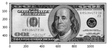
The imread () function of openCV is used to load an image from a file. Just pass as arguments the file path and the opening mode (grayscale or color).
img_dolar = cv2.imread("Fig0115(b)(100-dollars).tif", cv2.IMREAD_GRAYSCALE)
Image properties
img_dolar
array([[194, 194, 194, ..., 194, 194, 194],
       [194, 194, 194, ..., 194, 194, 194],
       [194, 194, 194, ..., 194, 194, 194],
       ...,
       [194, 194, 194, ..., 194, 194, 194],
       [194, 194, 194, ..., 194, 194, 194],
       [194, 194, 194, ..., 194, 194, 194]], dtype=uint8)
Note above that the loaded image is nothing more than a two-dimensional array. Each pixel is characterized by an coordinate (x, y) and an intensity value. The size of this matrix/image is determined by the number of columns/width (m) and rows/height (n) of the matrix (m x n).
img_dolar.shape
(500, 1192)
The image is 500 px high and 1192 px wide
img_dolar.max()
247
The maximum intensity value is 247.
YOU DO IT
Find the minimum and average value of the pixel intensity of the image.
# YOUR CODE HERE
Results:
Min: 0
Avg: 152.58884228187918
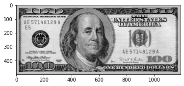
Showing an image
To view the representation of the actual image, not the matrix, we need to use the plt.imshow () function.
We pass as arguments the loaded image, the used color map and the minimum and maximum values that the pixels can assume.
plt.imshow(img_dolar, cmap='gray', vmin=0, vmax=255)
<matplotlib.image.AxesImage at 0x7f36775184e0>
Realize the need to inform the values of the parameters vmin and vmax. The minimum and maximum values expected for an 8-bit grayscale image are 0 and 255, respectively.
Caution: if vmin and vmax are not defined, matplotlib will set based on the values in the image and this may end up adjusting the contrast automatically.
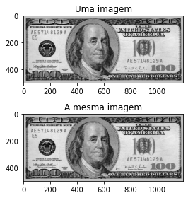
The use of subplots can help later when we need to make comparisons between images after some operations. Consult the [documentation] (https://matplotlib.org/3.3.3/api/_as_gen/matplotlib.pyplot.subplot.html) for a better understanding of the possible layouts.
plt.subplot(2,1,1) # 2 lines, 1 column, position 1
plt.title('An image')
plt.imshow(img_dolar, cmap='gray', vmin=0, vmax=255)

plt.subplot(2,1,2) # 2 lines, 1 column, position 2
plt.title('The same image')
plt.imshow(img_dolar, cmap='gray', vmin=0, vmax=255)

plt.tight_layout() # avoids overlapping image axes
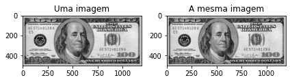
plt.subplot(1,2,1) # 1 lines, 2 columns, position 1
plt.title('Uma imagem')
plt.imshow(img_dolar, cmap='gray', vmin=0, vmax=255)

plt.subplot(1,2,2) # 1 lines, 2 columns, position 2
plt.title('A mesma imagem')
plt.imshow(img_dolar, cmap='gray', vmin=0, vmax=255)

plt.tight_layout() # avoids overlapping image axes
Basic operations with images
Selective cutting
As we saw earlier, images are represented by two-dimensional arrays. In that case, we can use the slicing properties of arrays in Python!
Making a slice means selecting the elements from one index to another in the array: my_array [start: end].
Since we are dealing with two-dimensional arrays, the start and end positions must be defined for both rows and columns: my_array[start: end, start: end]
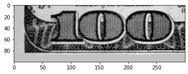
cut = img_dolar[400:500, 0:300]
plt.imshow(cut, cmap='gray', vmin=0, vmax=255)
<matplotlib.image.AxesImage at 0x7feed0873240>
YOU DO IT
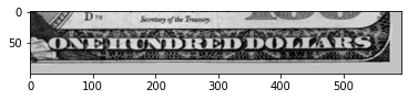
Slicing the region that contains the text “ONE HUNDRED DOLLARS” in the lower right corner of the image.
Tip: This is an approximate and manual process only. Observe the x and y axes of the original plotted image and try to find the approximate coordinate values for the region.
# YOUR CODE HERE
The final result should look like the image below:
<matplotlib.image.AxesImage at 0x7feed07af400>
Mirroring
To mirror images, we can also take advantage of the properties of an array by using a negative step (-1) to reverse the desired direction:
my_array[start: end, start: end: -1], will mirror the image horizontally
img_dolar_flip_horizontal = img_dolar_flip_horizontal[::,::-1]

plt.imshow(img_dolar_flip_horizontal, cmap='gray', vmin=0, vmax=255)
<matplotlib.image.AxesImage at 0x7f764811c668>
Another way is with the use of the flip () function of openCV:
img_dolar_flip_horizontal = cv2.flip(img_dolar, flipCode = 1)

plt.imshow(img_dolar_flip_horizontal, cmap = 'gray', vmin = 0, vmax = 255)
<matplotlib.image.AxesImage at 0x7f7651d7f358>

YOU DO IT
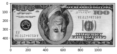
Perform vertical mirroring of the image.
# YOUR CODE HERE
Result:
<matplotlib.image.AxesImage at 0x7f76480fb0f0>
Rotation
The openCV package offers the rotate () function to rotate images.
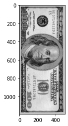
See below how to rotate 90º clockwise:
img_dolar_90_cw = cv2.rotate(img_dolar, cv2.ROTATE_90_CLOCKWISE)

plt.imshow(img_dolar_90_cw, cmap='gray', vmin=0, vmax=255)
<matplotlib.image.AxesImage at 0x7f7647e7e8d0>
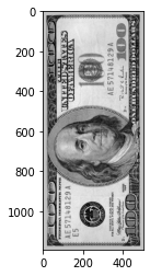
YOU DO IT
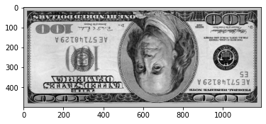
Perform 90º counterclockwise and 180º rotations of the image.
# YOUR CODE HERE
Result
plt.imshow(cv2.rotate(img_dolar, cv2.ROTATE_90_COUNTERCLOCKWISE), cmap='gray', vmin=0, vmax=255)
<matplotlib.image.AxesImage at 0x7f7647ddb588>
plt.imshow(cv2.rotate(img_dolar, cv2.ROTATE_180), cmap='gray', vmin=0, vmax=255)
<matplotlib.image.AxesImage at 0x7f7647db3358>